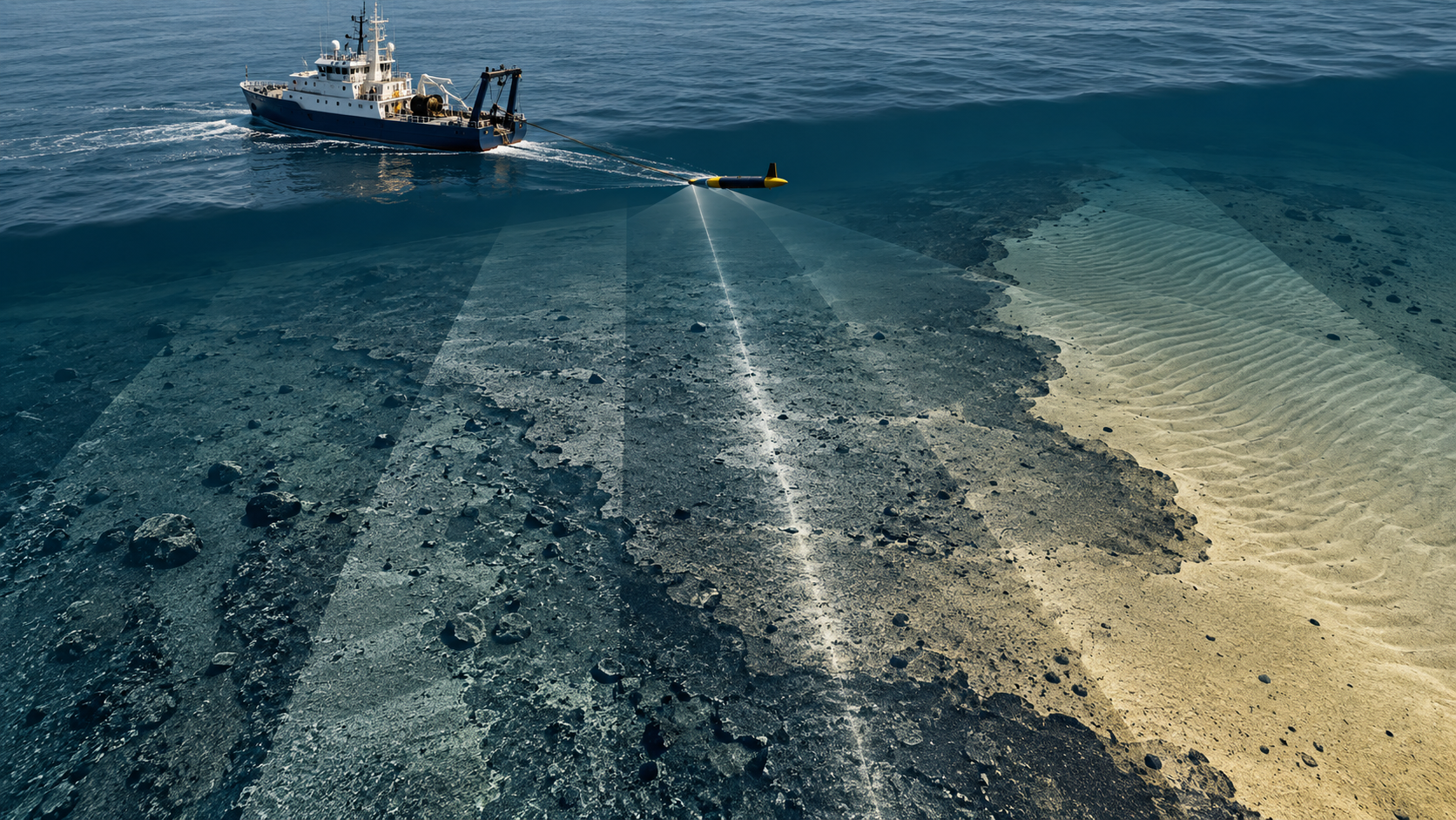
A side-scan sonar mosaic can look like a geological map even when its strongest boundary was made by the instrument. Here is a practical way to tell the two apart before a cable route or sediment map is approved.

The seam that looked like a sediment boundary

Imagine two adjacent side-scan sonar (SSS) lines across a proposed export-cable corridor. One line is visibly brighter on its outer range. A processing team joins the lines, draws a boundary between “coarse” and “fine” sediment, and recommends sampling on either side. Yet the boundary follows the edge of the swath, moves when the same area is viewed from the opposite direction, and disappears in the overlap. That is a processing hypothesis to test, not a geological contact to report.

Backscatter intensity is affected by grazing angle, range, absorption, source and receiver beam patterns, gain, fish altitude, seabed slope, and the sediment itself. The grey value in a delivered image is therefore not a direct measurement of grain size or strength. Blondel’s Handbook of Sidescan Sonar discusses the physics and processing of these returns. Johnson and Helferty’s geological interpretation paper makes a related point: display resolution, acoustic resolution and the actual geological information are different quantities. A more recent experimental study of SSS radiometric correction explicitly accounts for sediment variation instead of treating every brightness change as an illumination error.

Why blanket normalization can make matters worse

Time-varying gain tries to compensate for weaker returns with range. Slant-range correction moves returns from travel time to their estimated ground position. Neither step makes two images automatically comparable. A correction curve estimated from an entire swath may mix genuinely different seabed types. If a sand-to-gravel transition occupies the outer half, forcing its mean brightness to match the inner half can erase a real boundary. Conversely, an uncorrected beam-pattern or angle effect can manufacture one.

The first diagnostic is geometry. Preserve the original waterfall and its acquisition metadata. Map each suspect change against fish track, port or starboard side, altitude, range, grazing angle, gain setting, and line number. A tonal edge parallel to a track or repeated at the same fractional range on several lines deserves particular scrutiny. A boundary that cuts independently across tracks and is reproduced in overlapping coverage is more credible, although still not a sediment classification.

A reproducible five-stage QC workflow

1. Separate geometric from radiometric corrections. Confirm seabed pick, fish altitude and slant-range conversion on individual lines. Inspect whether a misplaced bottom track has stretched or compressed the near range. Record towfish navigation and latency assumptions before mosaicking.

2. Compare like with like. Select overlapping patches of apparently uniform bottom and compare their return distributions within similar range and incidence-angle bands. Avoid matching a near-range sample to a far-range sample without an angle-aware correction. Keep source-line IDs in the final mosaic so every suspect patch can be traced back to raw data.

3. Estimate corrections without flattening geology. Use a reference patch or sediment-stratified approach, and exclude obvious boulders, shadows, nadir and boundaries from the correction estimate. Apply the candidate correction to withheld lines. If it improves seams but erases repeatable geological texture, reject or revise it.

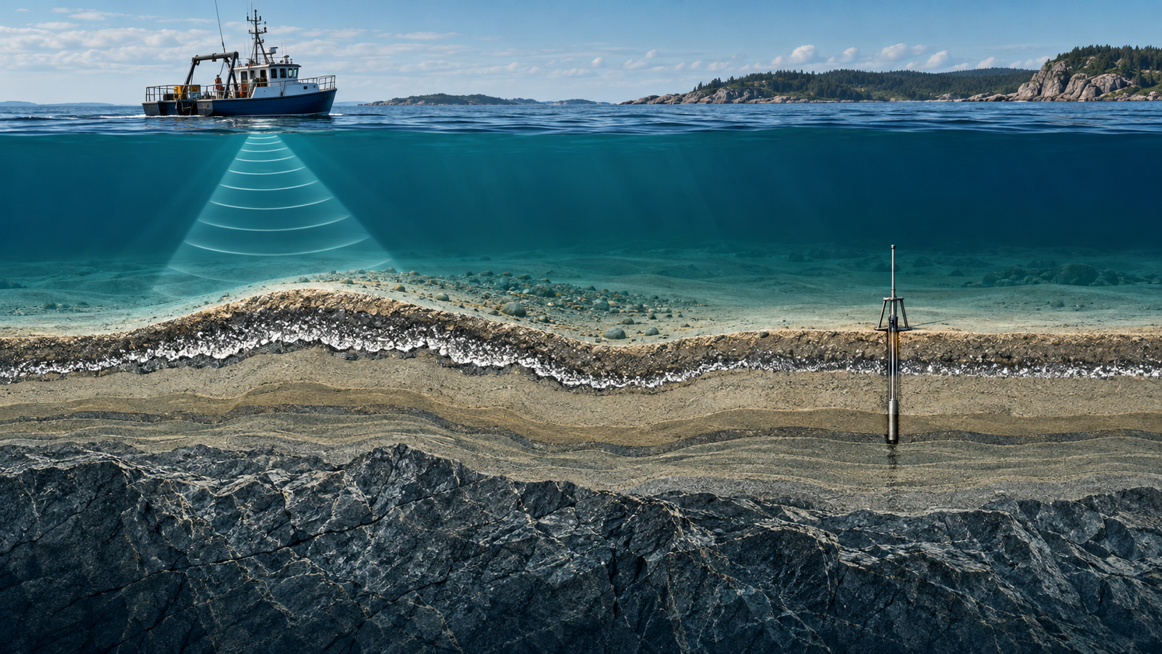
4. Validate independently. Overlay multibeam bathymetry and backscatter, sediment samples, photographs or video where available. A core or grab establishes material at a point; it does not automatically calibrate every pixel between points. Sample both sides of a persistent boundary, and also sample an apparent boundary that the processing says is an artefact. This is a useful test of the method.

5. Deliver uncertainty with the map. Provide the raw-line comparison, a corrected mosaic, a footprint or coverage layer, validation points, and a confidence layer. Classify “acoustic facies” first; assign material names only where observations support them.

Worked decision example

Suppose a 200 m-wide corridor is crossed by two opposing SSS lines. A bright strip appears 60–90 m from the towfish on the first pass. On the reciprocal line, brightness follows that line’s outer range instead of the same seabed position. In their overlap, the same patch is bright in one direction and moderate in the other. The repeatability test fails: do not map a gravel boundary from the strip. Recheck altitude, gain history and angle response, then compare the corrected reciprocal coverage. A small grab-and-video plan can target the remaining ambiguity. The distances here are illustrative workflow values, not a reported GeoSubsea survey.

If, after correction, an edge remains fixed geographically, crosses both swaths and coincides with a change in seabed texture and samples, it becomes a defensible acoustic facies boundary. Still describe the sampling support and interpolation distance. A neat seam-free mosaic is a visual product; the engineering product is a traceable interpretation.

What an expert review should reject

Reject a map based only on a histogram-stretched final mosaic; an unexplained brightness-to-lithology lookup; a boundary drawn along an acquisition line; or a classification accuracy estimated from samples used to tune the correction itself. Also reject a QC report that calls every dark patch soft mud: shadow, slope, nadir and gain can all make darkness. If an algorithm or AI classifier is used, reserve whole survey lines or a different area for independent validation. Random neighboring pixels are too similar to demonstrate real transfer performance.

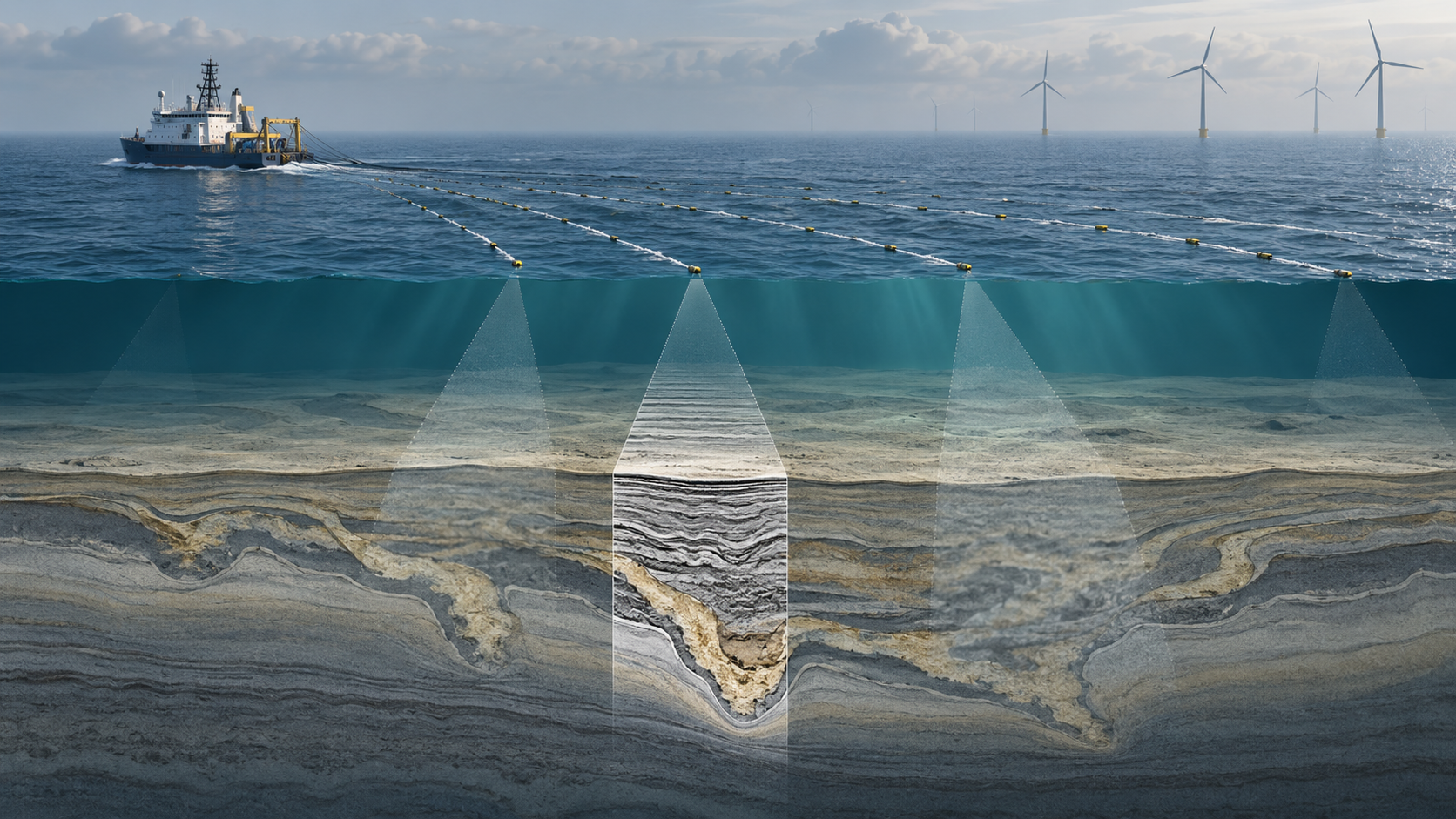
The best correction preserves known contrasts while removing acquisition imprint. For a cable project, that means pairing SSS with samples and the relevant SBP and MBES data, then documenting where interpretation remains uncertain. That is more useful than a visually perfect image whose sediment labels cannot survive a reciprocal line check.

References

Blondel, P. (2009), The Handbook of Sidescan Sonar, Springer-Praxis; Johnson, H. P. and Helferty, M., The Geological Interpretation of Side-Scan Sonar (both supplied as background reading). Li et al., “A New Radiometric Correction Method for Side-Scan Sonar Images in Consideration of Seabed Sediment Variation,” Remote Sensing 9, 575 (2017): original research. For an independent empirical connection between SSS returns and shallow sediment properties, see Geo-Marine Letters (2023). This article proposes a QC workflow; its numerical example is illustrative.