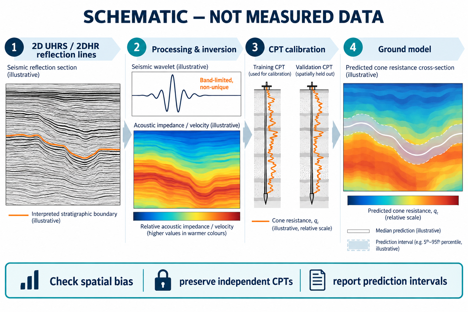
A seismic line can cross a wind-farm lease area every few hundred metres, while cone penetration tests (CPTs) remain discrete, expensive measurements. That mismatch makes machine-learning predictions of cone resistance between tests attractive for cable corridor and foundation ground models. But a continuous colour volume can look more certain than the evidence behind it. The practical question is not whether a model can draw a dense grid; it is whether its predictions are calibrated, spatially validated and useful at the scale of the engineering decision.

What the new work shows—and what it does not

A recent open-access research article by Dongfang Qu, published online on 25 September 2026 in Geodata and AI, integrates seismic reflection data and CPT data to predict spatially continuous CPT parameters at offshore wind sites. It reports that interpreted stratigraphic units or seismic attributes can add value where the other input does not resolve subsurface variability, and that the contribution of coordinates depends on CPT spacing relative to the scale of lateral change. The author also describes seismic data quality as affecting the geological detail captured, while noting this as a preliminary qualitative observation. The underlying data are confidential, so readers cannot independently reproduce the site examples from the paper.

Qu’s paper is a journal research article, available as an in-press corrected proof, not a preprint. Its confidential data limit independent reproduction. The results show active development, not a universal conversion from seismic amplitude to cone resistance or evidence that predicted CPTs can replace direct tests.

Why reflection data cannot uniquely determine qc

Reflection seismic records changes in acoustic impedance, the product of density and compressional-wave velocity. After processing, inversion estimates a band-limited impedance model subject to a wavelet, starting model, regularization and assumptions about noise. The mapping from impedance or velocity to cone resistance qc is indirect. Soil fabric, stress history, saturation, cementation, grain size and thin layering can produce different geotechnical responses even where seismic properties appear similar. Conversely, a thin weak layer may matter to a cable trench or pile but fall below seismic resolution.

For 2D high-resolution or ultra-high-resolution seismic (2DHR/UHRS), start with acquisition QC: source signature and timing, navigation and receiver geometry, tide and sound-velocity corrections, line positioning and crossover repeatability. Review gathers for bubble pulses, ghosting, swell noise, multiples, dropouts and acquisition footprint. A high-resolution display does not guarantee high vertical resolution; bandwidth, signal-to-noise ratio, migration velocity and wavelet control which interfaces are separable. Preserve processing versions and flag weak or uncertain responses.

Make CPT calibration traceable

Before training, check CPT coordinates and vertical datum, penetration depth, cone area ratio and correction status, units, test type, refusal, dissipation or pore-pressure channel quality, and any changes between field campaigns. Do not silently merge corrected and uncorrected sleeve friction or cone resistance. Keep the raw log, processing history and selection mask so an engineer can trace each model input to its source. This is not paperwork: a questionable calibration point can pull a regression toward a spurious relation.

Use geological interpretation as an explicit model input or stratification where it is defensible, rather than assuming one relation applies across every depositional unit. The model should document which seismic attributes, interpreted horizons, facies and CPT parameters are used, at what support or vertical averaging, and with what coordinate reference. Upscaling a centimetre-scale CPT log to seismic support may reduce resolution mismatch, but it cannot create information; report the averaging window and test its effect.

The 2025 Integrated Ground Model report for RVO’s Nederwiek Wind Farm Zone Site I gives a useful real-world example of this discipline. Its quantitative prediction workflow combined geotechnical and geophysical data, geostatistical elastic priors, wavelet estimation and 2D UHRS pre-stack inversion, with uncertainty estimation and comparison against ground-truthed data. The report lists 114 seabed CPTs, 59 downhole CPTs and 42 SCPTs, and flags reliability concerns in sleeve friction at selected locations; corrected values were used at 16 locations under the contractor’s procedure. These counts and decisions describe that project only, not a recommended minimum or a transferable performance benchmark.

Validation must respect geography

A random train/test split can make a spatial model appear accurate when nearby CPTs share the same geology and seismic footprint. Instead, reserve spatially separated CPTs or whole line segments before model fitting. Where the project allows, test performance in more than one geological unit and at the edges of the survey area, where extrapolation is most likely. Report errors by parameter, depth interval and unit, alongside bias and prediction-interval coverage. Compare against simple baselines, such as nearest-neighbour or unit-wise statistics, so added model complexity earns its place.

Do not tune against the hold-out CPTs. Report their number and distribution, distance to the nearest training CPT and coverage of conditions relevant to the route or foundation. Error and uncertainty maps are more diagnostic than one site-wide score.

Turn uncertainty into an action

Prediction intervals should travel with the median estimate into the interpreted section, GIS layer and ground model. Separate measurement uncertainty from processing and inversion uncertainty, calibration scatter, model uncertainty and spatial extrapolation where possible. A narrow interval does not guarantee accuracy if the model is biased or its calibration domain is wrong. Check interval coverage on independent CPTs and identify areas where the model is outside its training range.

For cable routing, these outputs can prioritize additional investigation: a predicted weak or variable layer near a crossing may justify a targeted CPT, borehole, vibrocore or higher-density seismic tie, subject to project requirements. A high-uncertainty zone may be more important than a low median qc. For a foundation or trench design, take characteristic parameters and acceptance decisions through the project’s geotechnical design basis and responsible engineer; do not feed an unqualified ML prediction directly into design.

A practical release checklist

• Trace every input to a coordinate, datum, test record and processing version.
• Review seismic bandwidth, noise, wavelet and line ties before attributing fine detail to inversion.
• Keep spatially independent CPTs out of feature selection and model fitting.
• Report validation distribution, bias, interval coverage and performance by geological unit.
• Map extrapolation and uncertainty, and link those areas to proportionate follow-up investigation.
• Label predicted CPTs as predictions in every figure, GIS layer and deliverable.

Machine learning can help carry sparse geotechnical measurements between seismic lines, but its value comes from a defensible integration workflow, not the density of the output grid. For offshore cable and wind-farm decisions, the reliable product is a traceable ground model that shows where the data support an interpretation, where they do not, and what investigation would reduce the remaining uncertainty.

References

• Qu, D. (2026). Quantitative ground modelling integrating geophysical and geotechnical data using machine learning. Geodata and AI, 100122. Available online 25 September 2026; in-press corrected proof. Research article, not a preprint.
• Rijksdienst voor Ondernemend Nederland (RVO) (2025). Nederwiek Wind Farm Zone Site I Integrated Ground Model Report, 27 June 2025.
• Rizzuti, G., Telling, R. & Vasconcelos, I. (2024). Deep-learning-based uncertainty quantification for post-stack UHR seismic inversion. EAGE GET2024 Offshore Wind Energy Conference contribution.