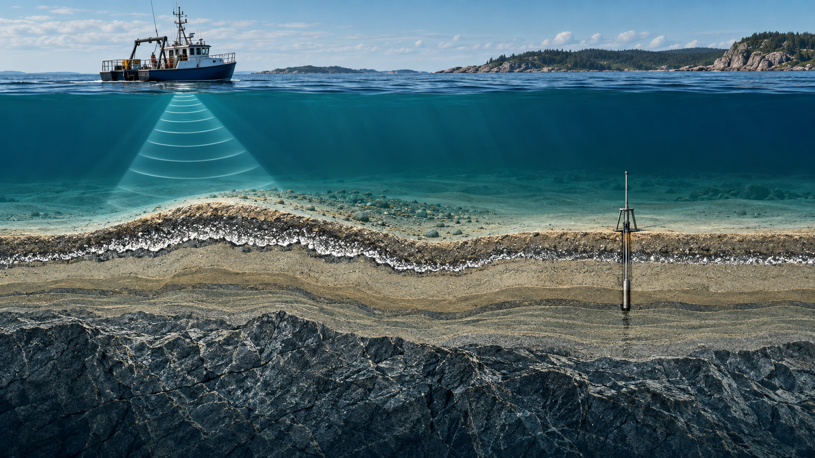
A bright, shallow sub-bottom reflector may mark a stiff layer, shell lag, peat, gravel or bedrock. Treating one strong line as “rock” can change a cable-burial plan before the ground model is ready.

The practical problem

A chirp or pinger profile shows a clear seabed and a strong reflector 1.5 m below it along part of a cable corridor. Below that line, the image fades. Does the cable encounter rock at 1.5 m? The honest answer is that an acoustic contrast is present at an estimated depth. The reflector’s material, continuity and excavability are separate questions. A high-amplitude return may represent a large impedance contrast, strong attenuation below a coarse layer, tuning between thin interfaces, or acquisition artefacts. None by itself proves bedrock.

This distinction matters because the engineering decision is about achievable depth of lowering, thermal environment and trenching risk. An interpreted horizon must be connected to samples, cone penetration tests (CPTs) or other appropriate ground truth before it becomes a lithological surface. Recent work using a three-dimensional acoustic profiler alongside cable tracking reports that shallow soil changes can help explain variable burial and trenching difficulties. That is a useful application, but its observations should not be generalized to every SBP frequency or soil type.

What the instrument actually measures

SBP records acoustic arrivals in two-way travel time. To convert an interpreted separation Δt to thickness, use h = vΔt/2, where v is the acoustic velocity assigned to the interval. If Δt is 2 ms, v = 1,500 m/s gives 1.50 m; v = 1,700 m/s gives 1.70 m. The 0.20 m spread is a velocity sensitivity, not necessarily the full uncertainty. Picking, tidal or heave correction, seabed tracking and phase or wavelet character also matter. Never print a thickness with centimetre precision simply because the display cursor offers it.

Vertical resolution depends on the effective bandwidth and wavelet after processing. Two closely spaced interfaces can interfere, making one composite bright event. A thin sand layer between cohesive units may thus look like a single hard boundary. Conversely, penetration can stop beneath coarse, gas-bearing or attenuating sediment while a deeper interface remains present but invisible. “No deeper reflector observed” is an observation; “bedrock directly below” is an inference that needs separate evidence.

A route-screening workflow

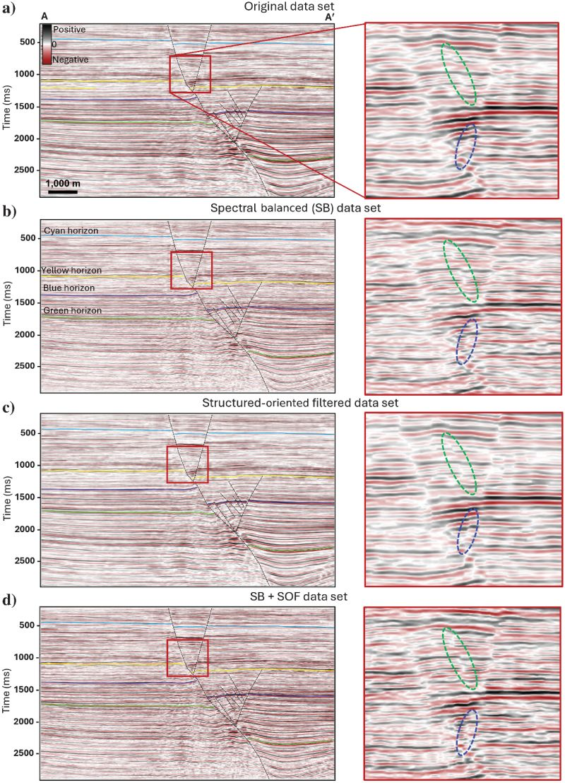
Preserve the raw acoustic character. Review raw and processed records side by side, including pulse settings, gain and filter history. A ringing event tied to the seabed at nearly constant delay can imitate a parallel geological reflector. Check whether it changes with acquisition settings, depth or seabed slope. Inspect crossings for consistent two-way time and phase.

Pick more than a single line. Interpret seabed, the first reliable sub-bottom event, and the zone of lost penetration separately. Record each horizon’s pick quality and terminate it at gaps. Do not bridge an unobserved interval merely to draw a continuous coloured surface. Map thickness only where both top and base have support.

Calibrate with targeted intrusive data. Place CPTs and cores where the strong event first appears, where it disappears, and where predicted burial risk is highest. Compare the reflector depth with stratigraphic logs and cone resistance, allowing for navigation error and vertical datum. A high cone resistance interval is not a rock identification by itself; review core material, recovery and the entire profile.

State alternative models. At each critical segment, write down at least two plausible interpretations: for example a coarse lag over soft sediment versus a weathered rock surface. Ask what survey or sample would discriminate between them. Test cable burial options against both models until the difference is resolved.

Illustrative design decision

Consider a corridor where a bright event lies 1.2–1.8 m below seabed on five lines. Two crossings agree, but one crossing shows a 0.4 m offset after heave correction. An adjacent CPT records a stiff interval starting at 1.4 m; a core, however, contains gravel over consolidated clay and no bedrock. The correct report is a laterally variable stiff or coarse shallow unit, with uncertainty at the crossing and limited penetration below. Calling the whole horizon “bedrock” would overstate the evidence. The values are hypothetical, used to show the decision sequence.

Now suppose the installation target is 1.5 m of cover. The uncertain base crosses that threshold. The next action is not to average the depths and declare the route acceptable. Investigate the crossing, sample the pinch point and ask the burial engineer whether a lower confidence bound on achievable cover changes the tool or protection method. An uncertainty of a few decimetres matters when it straddles the design decision.

What to put in the deliverable

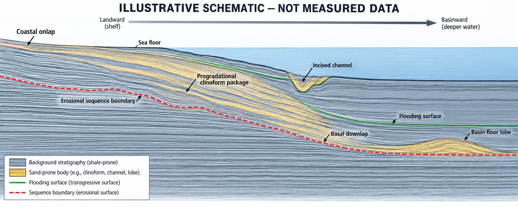
Supply annotated examples of raw and processed SBP records; time-domain picks; velocity assumptions and a sensitivity table; sample and CPT tie panels; line-crossing residuals; maps showing observed versus interpolated horizons; and a short risk register linked to proposed verification locations. Separate acoustic facies from geological units and engineering properties. The former can be mapped continuously where the signal is clear; the latter require calibration.

This approach turns a striking reflector into a testable ground model. It also prevents a common mistake: using a beautifully continuous SBP image as a substitute for a verified statement about excavability or cable cover.

References

Griffiths and Noel, “Understanding the Effects of Shallow Soils on Sub-seabed Cables Using a 3D Acoustic Profiler”, EAGE GET 2024. GEUS, “Seismic imaging of shallow marine sediments offshore Denmark using ultra-high resolution multi-channel seismic data” (2024). The example above is illustrative; this article does not report a GeoSubsea project.