Can Legacy 4 kHz SBP Data Screen Offshore Cable Routes? Evidence from 506 Irish Survey Lines

A legacy sub-bottom profiler (SBP) archive can be valuable before an offshore wind developer commissions a new cable-route survey. It can reveal where a shallow sediment package is visible, where buried channels may offer a different corridor, and where interpretation fails. But it cannot certify burial depth or trenchability. A 2026 Irish study offers an unusually useful test of that distinction: researchers reprocessed 506 existing SBP lines and reported both measurable route outcomes and the limitations of the old data.

What the Irish study actually analysed

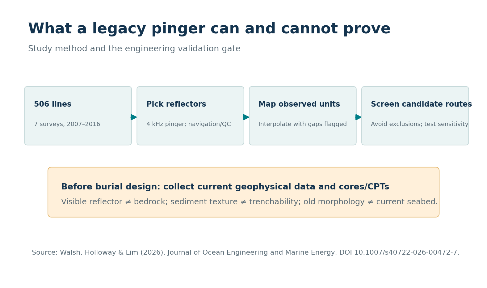
Walsh, Holloway and Lim examined potential submarine export cable routes around the South Coast Designated Maritime Area Plan (DMAP). For the Waterford and Wexford subareas, they used 506 SBP lines from seven INFOMAR surveys acquired between 2007 and 2016. The cited pinger was a 4 kHz SES 5000 array. The team refined navigation, tracked the seabed, adjusted display gains, picked reflectors and interpolated interpreted sediment-thickness points into a route-screening surface. This was a feasibility-stage GIS study, not a construction survey or a GeoSubsea project.

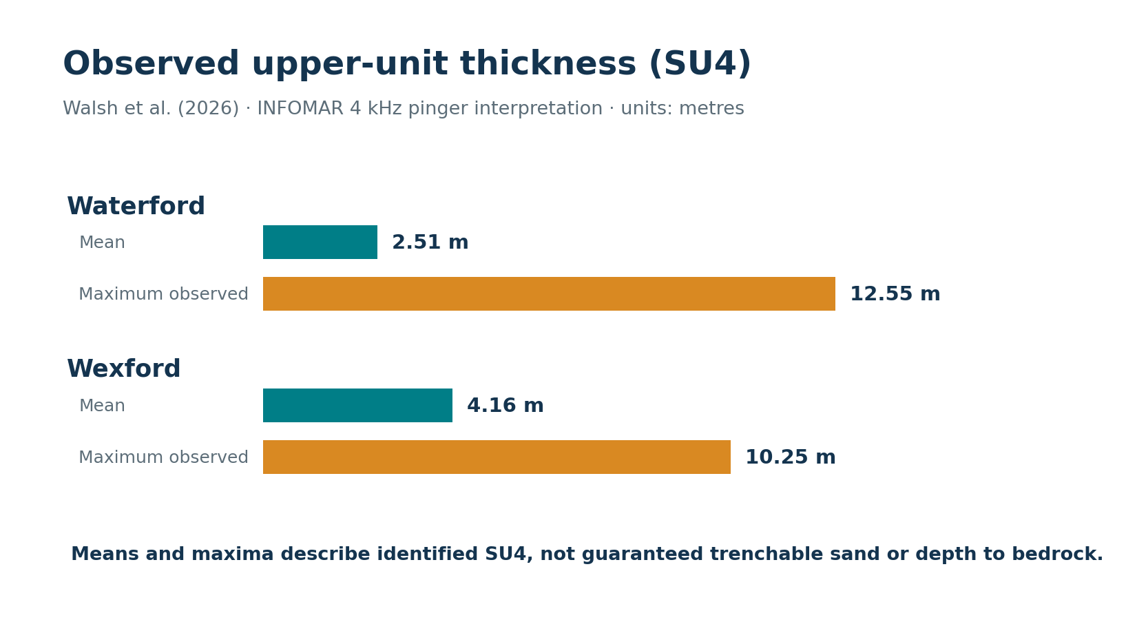
The uppermost interpreted unit, SU4, appeared as low-amplitude, approximately parallel layering. INFOMAR seabed samples associated with that unit indicated sand, gravelly sand or sandy gravel. In Waterford, the paper reports a mean visible SU4 thickness of 2.51 m and a maximum of 12.55 m. In Wexford, the corresponding values are 4.16 m and 10.25 m. The Wexford mean is 1.65 m greater, but that regional contrast cannot predict the thickness beneath one proposed cable chainage. A maximum observed value is especially poor evidence for a minimum continuous burial corridor.

Waterford SU4 mean 2.51 metres and maximum 12.55; Wexford mean 4.16 and maximum 10.25, as published by Walsh and colleagues in 2026. — Figure 1. Reported thickness of the identified upper seismic unit SU4. Data: Walsh et al. (2026); means and maxima are not minimum continuous burial thicknesses.

The interpretation that must not be skipped

The researchers did not equate every picked basal reflector with bedrock. Their interpolation used the greatest identifiable thickness for each unit, and the paper explicitly warns that the resulting value is usually not depth to bedrock. R1 was interpreted as possible buried bedrock or glacial till, but was rarely seen with the low-penetration pinger. A reflector may mark a change in acoustic impedance within workable sediment; absence of a deeper reflector can simply mean the instrument stopped seeing it. Calling these grids “bedrock depth” would convert a cautious observation into a false engineering fact.

Likewise, an acoustic label such as “sand” does not tell an installer how a specific plough, jet trencher or mechanical trencher will perform. Gravel content, density, cementation and cobbles matter. A seismic unit is a geological interpretation; trenchability requires geotechnical tests and tool-specific assessment. Keep separate GIS layers for the picked two-way times, assumed velocities, converted thickness, acoustic-data quality and ground-truth evidence. Flag blank zones rather than filling them with apparently confident colours.

What changed in route screening?

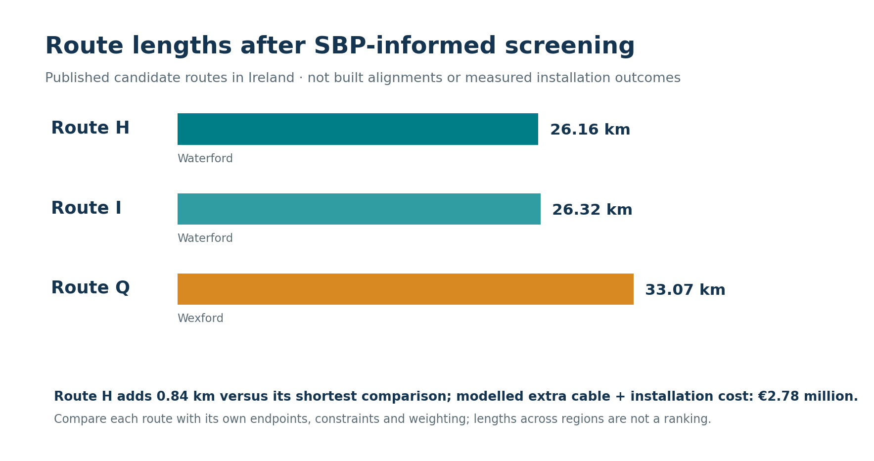
The study combined sediment-thickness surfaces with protected areas and exclusion zones in a least-cost-path analysis. In Waterford, Routes H and I scored 1.18 each on the paper’s normalized 1–5 suitability scale and measured 26.16 km and 26.32 km. In Wexford, Routes Q and R scored 1.14 and 1.20; Route Q measured 33.07 km. These are candidate paths under the authors’ weighting and endpoints. Comparing Q’s length directly with H’s would be misleading because they serve different geographic connections. A low suitability cost is also a GIS score, not an invoice.

The authors estimate that optimized Route H adds 0.84 km relative to its shortest comparison and model an extra €2.78 million in cable and installation costs using the cited cost assumptions. That is a real published model result, not an observed project overrun or a universal price per kilometre. The practical trade-off is clear: a slightly longer path can screen out poor ground or conflicts, but a project team must re-run costs with its own voltage, cable, installation method, landfall and exclusions.

Published candidate route lengths are H 26.16 kilometres, I 26.32 kilometres and Q 33.07 kilometres; H has a modelled 0.84 kilometre addition. — Figure 2. Candidate route lengths reported by Walsh et al. (2026). Waterford and Wexford routes have different endpoints; the €2.78 million figure is a model estimate for Route H, not a measured installation cost.

A defensible way to reuse an old pinger archive

Begin with the original line locations, navigation quality, datum and acquisition metadata. Identify which profiles actually cross the candidate corridors. Reprocess from raw records where possible and review seabed tracking, gain effects, multiples and penetration line by line. Tie horizons at line intersections and record contradictory picks. Depth conversion must carry a velocity range, not only one nominal value; any thickness interpolated between sparse lines needs an uncertainty or data-density flag.

Next, make two maps: observed acoustic evidence and route decisions. The first should show surveyed versus interpolated areas, reflector continuity, samples and alternative interpretations. The second can screen several feasible paths against environmental exclusions, seabed conditions and likely engineering constraints. Test how rankings change when the sediment weighting, velocity, missing-data treatment and exclusion buffers change. A route that wins only under one optimistic assumption is not robust.

Finally, specify a targeted modern survey and sampling plan. Re-survey mobile areas with current MBES and, where useful, side-scan sonar; acquire higher-quality SBP or ultra-high-resolution seismic across thin or ambiguous cover; place cores and cone penetration tests at apparent pinch points and facies boundaries. Use the resulting ground model for a project-specific cable burial risk assessment. The 2026 paper notes that its 2007–2016 SBP and 100 m GIS grid are appropriate for feasibility screening, not detailed installation design.

Workflow uses 506 legacy pinger lines for reflector picks and feasibility screening, then requires current geophysical surveys and geotechnical validation before burial design. — Figure 3. A practical validation gate derived from the study method and its stated limits. This is an editorial workflow diagram, not a figure reproduced from the paper.

The useful lesson

Legacy data reduce uncertainty early only when their limits travel with the map. Here, 506 real lines exposed substantial variation in the upper unit and helped identify candidate corridors, while older acquisition dates, incomplete penetration and coarse grid cells prevented any claim of guaranteed burial performance. The expert deliverable is therefore a shortlist plus a clear plan to test its weakest assumptions, not a definitive trench depth inferred from a coloured raster.

Source

Walsh, K., Holloway, P. and Lim, A. (2026), “Optimising submarine cable routes from offshore wind farms,” Journal of Ocean Engineering and Marine Energy, DOI: 10.1007/s40722-026-00472-7. Figures 1–2 redraw numerical results reported in the paper; Figure 3 summarises an interpretation workflow. No project data from GeoSubsea are implied.