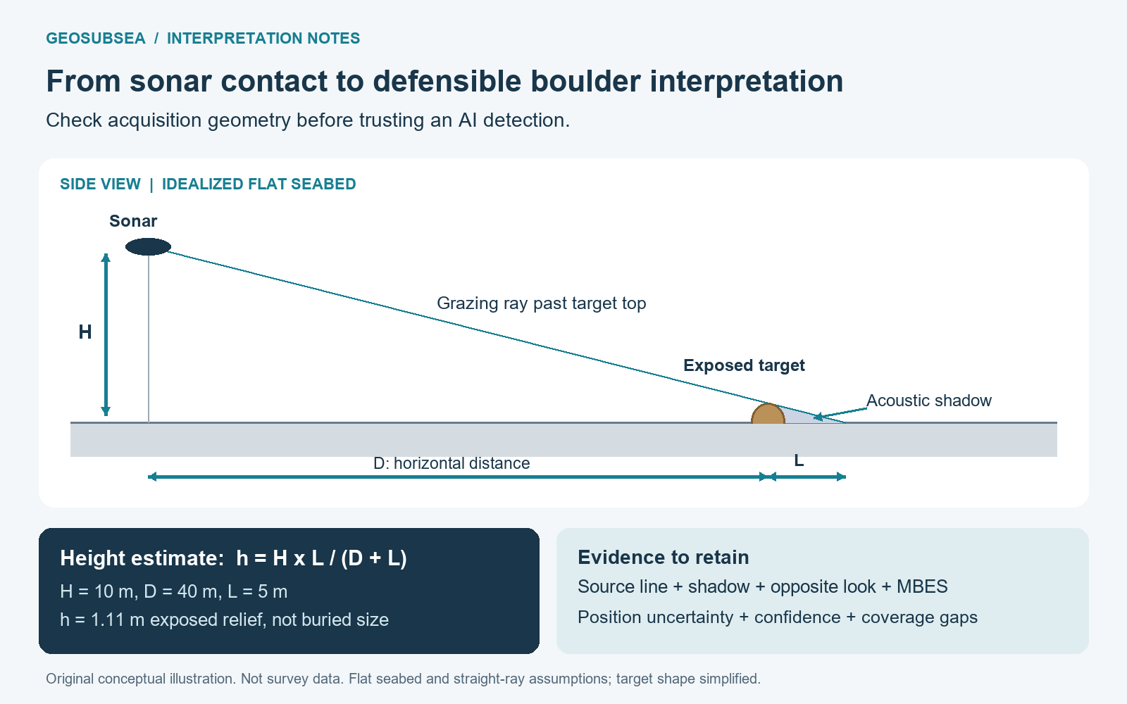
A boulder contact list can influence cable micro-routing, pre-lay clearance and installation planning. Yet a clean side-scan sonar (SSS) mosaic does not, by itself, establish that every relevant obstruction has been detected or correctly positioned. The practical challenge is to turn acoustic evidence into a traceable interpretation while preserving the uncertainty that matters to the engineer.

AI-assisted detection makes this particularly timely. At the 2025 UK Marine Technology Postgraduate Conference, Michal Motylinski presented a workflow combining boulder detection, duplicate removal and target–shadow separation. It illustrates active progress in automation, rather than a universal performance guarantee. For a cable-route survey, the useful question is how well a detector performs on the actual seabed, acquisition geometry and minimum target size required by the project. [1]

Start with detectable targets, not mosaic pixel size

A 0.10 m mosaic cell is a display and resampling choice; it is not evidence of 0.10 m object resolution. Sonar frequency, pulse characteristics, beam footprint, range, altitude, tow speed and ping spacing constrain what the acquisition can resolve. Johnson and Helferty also distinguish resolution from detectability: an isolated, high-contrast object may be detectable without its dimensions being reliably resolved. [2]

Before interpretation, define the target dimensions and exposed relief relevant to the installation method. Check representative contacts across near, middle and far range, including rough seabed. Map unusable nadir, outer-range degradation, dropouts and turn-related gaps. Nominal swath overlap is insufficient if both observations provide poor target visibility. Where practical, acquire an independent look direction to reduce ambiguity from shadows and seabed texture.

Correct geometry before classifying contacts

Validate timestamps, coordinate reference systems, sensor offsets, towfish positioning and altitude picks before measuring targets. Vessel GNSS accuracy does not describe the complete uncertainty of a towed sonar contact. Layback assumptions, cross-current displacement and heading errors can separate two observations of the same object or make unrelated objects appear coincident.

For a flat seabed and straight sound path, ground range is x = √(r² − H²), where r is slant range and H is sonar altitude. An incorrect bottom pick therefore affects target location and dimensions. On sloping or irregular terrain, this flat-bottom approximation becomes less reliable; suitably registered bathymetry helps identify where terrain effects require attention. Blondel describes these geometric corrections and their associated artifacts in detail. [3]

Keep an auditable processing sequence. Review gain and beam-pattern corrections, along-track scaling and contrast adjustments against the source records. Avoid clipping strong returns or filtering away small targets. A visually uniform mosaic is useful for regional interpretation, but seam selection and blending can weaken or remove the clearest observation of a contact. Retain the original line and ping reference for every interpreted target.

Read the return and its shadow together

Interpret a candidate using its acoustic return, shadow, shape, surrounding texture and repeat observations. Display polarity must be known: a dark patch is not automatically a shadow. Ripple troughs, small scarps and processing artifacts can resemble isolated objects; a bright return alone cannot establish that the target is rock.

A simple geometric example shows why measurement definitions matter. Let H be sonar altitude, D the horizontal distance to an idealized target’s shadow-casting point, and L the horizontal shadow length beyond that point. On a flat seabed, similar triangles give h = HL/(D + L). For H = 10 m, D = 40 m and L = 5 m, the estimated exposed height is 1.11 m. This is a hypothetical calculation, not a project observation.

The estimate assumes a clear shadow endpoint, a straight grazing ray and simplified target geometry. Seabed slope, an irregular boulder, partial burial and overlapping shadows can invalidate those assumptions. Report exposed relief separately from plan dimensions, and never equate acoustic height with the boulder’s full buried size.

Validate AI on independent survey areas

Use automated detections as candidates for review. A model confidence score is not automatically a calibrated probability that a contact is a boulder. Performance may change with sonar settings, substrate, range, image normalization and target density.

Recent research on multibeam point clouds also demonstrates the difficulty of transferring models from synthetic to real sonar data. That 2025 preprint concerns a different sensor representation and target task; its numerical results should not be presented as SSS boulder-detection performance. It nevertheless provides a relevant warning about assuming that training conditions represent production data. [4]

A practical validation plan should hold out complete lines or spatial areas, avoiding overlapping views of the same boulder in both training and testing. Use independently reviewed labels and report precision, recall and missed targets by size class, range and seabed type. Include manual review of selected areas where the model found nothing. Reviewing only detected boxes cannot reveal false negatives.

Set acceptance criteria before production. Retain model version, preprocessing settings, detection threshold and reviewer decisions. During duplicate reconciliation, compare position uncertainty, geometry and source images; a fixed distance threshold can incorrectly merge neighboring boulders in a dense field.

Integrate the evidence before making a route recommendation

MBES can test whether a contact has measurable relief, provided its footprint and sounding density support that comparison. Absence from a coarse bathymetric grid does not disprove an SSS contact. SBP and 2D high-resolution seismic add shallow stratigraphic context, such as sediment cover or a possible coarse deposit, but do not automatically confirm every buried boulder.

Keep observations separate from interpretations in the contact register. Record source line, position and uncertainty, dimensions, height method, classification confidence, supporting datasets and unresolved alternatives. Distinguish an area with no interpreted contacts from an area with inadequate detection coverage. Where the remaining uncertainty affects routing or clearance, recommend targeted reacquisition or appropriate visual investigation.

The strongest deliverable is a defensible evidence trail: a reviewer can return from a mapped contact to the acquisition record and understand both the interpretation and its limits. This is where careful SSS processing, integrated interpretation and reporting add value beyond a convincing image. Explore GeoSubsea’s SSS processing and interpretation and integrated geophysical reporting services.

References

1. Motylinski, M. (2025). “Automatic Seafloor Boulder Detection in Side-Scan Sonar Imagery.” 8th UK Marine Technology Postgraduate Conference, presentation abstracts, p. 8. Conference abstract.
2. Johnson, H. P., and Helferty, M. (1990). “The Geological Interpretation of Side-Scan Sonar.” Reviews of Geophysics, 28(4), 357–380. See discussions of resolution, target detectability and image processing.
3. Blondel, P. (2009). The Handbook of Sidescan Sonar. Springer/Praxis. Chapters 3–4 and 10.
4. Shaukat, M. S., Käckenmeister, Y., Bader, S., and Kirste, T. (2025). “Towards Training-Free Underwater 3D Object Detection from Sonar Point Clouds: A Comparison of Traditional and Deep Learning Approaches.” arXiv:2508.18293, preprint.