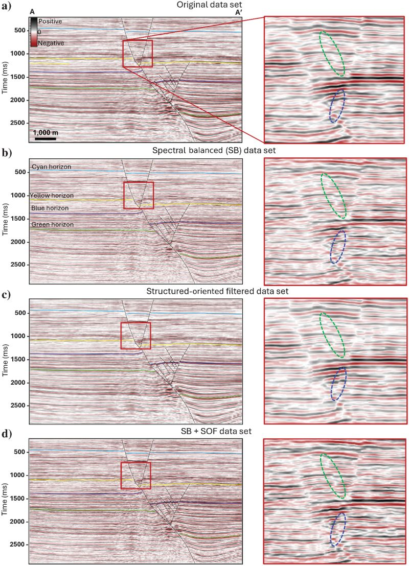
This case study summarizes a published post-migration conditioning workflow using the user-supplied figure, retained unchanged. It depicts study data, not a GeoSubsea or offshore-wind survey; route and ground-model implications below are general applications.

Figure 1. Line AA′ through the original, spectrally balanced (SB), structure-oriented filtered (SOF), and combined SB + SOF volumes. Green and blue ellipses highlight two fault examples. Figure supplied by the author and reproduced unchanged.

The seam is where interpretation gets tested

Two neighboring seismic surveys can look like different worlds after acquisition with different geometry, bandwidth, fold, processing, migration velocity, or display scaling. At the join, a horizon can appear to change amplitude or continuity abruptly. Is that a fault or stratigraphic edge—or a survey boundary?

The published example behind the figure tackles this problem in a merged post-migration dataset. It applies spectral balancing (SB), then structure-oriented filtering (SOF), and compares the original, each intermediate volume, and the combined result along line AA′. In the enlarged panels, green and blue ellipses draw attention to two fault responses. The comparison makes a valuable point: conditioning can make a structural interpretation more coherent across a seam, but no single enhanced panel is automatically the “truth.”

What each step changes

Original volume (a): This remains the reference. Frequency content may vary across the merge, and a narrowband patch may show a stratigraphic edge clearly near its tuning frequency. Preserve it as the control for every enhancement.

Spectral balancing (b): SB rescales parts of the recorded spectrum to reduce frequency imbalance. A more even spectrum can sharpen closely spaced reflectors and help follow horizons across the seam. It does not manufacture reliable earth information outside the recorded bandwidth. Where signal energy is weak, boosting a band can also lift noise, acquisition footprint, ringing, or residual migration artifacts. That distinction is central: a brighter, crisper trace is not necessarily a more accurate trace.

Structure-oriented filtering (c): SOF estimates local reflector orientation and smooths preferentially along those reflectors, while reducing incoherent and cross-cutting energy. Properly tuned, it clarifies continuity and fault displacement. Its steering depends on the dip estimate: If a fault-plane reflection, footprint, or migration artifact controls the local dip, the filter may follow the wrong event. A narrow fault can be softened, a true stratigraphic discontinuity can be smeared, or an artifact can become visually organized.

Combined SB + SOF (d): The authors report improved apparent vertical resolution within the signal-supported bandwidth, and clearer lateral delineation of fault and stratigraphic edges, with a more consistent interpretation across the merged seam. The enlarged fault panels allow direct comparison. The study also found that broader frequency content made noise and acquisition footprint more conspicuous, while SB sometimes diminished edges well imaged in the original narrowband volume. The balance is therefore local and geological, not merely cosmetic.

Why it matters for a marine route or wind-farm ground model

In a regional framework for a cable corridor or wind lease, a seam-induced break could create a false fault or split a horizon; smoothing could hide a real boundary that should guide follow-up lines or ground truth.

This affects survey planning, not engineering predictions. A conditioned seismic image cannot by itself assign soil strength, sediment type, cable burial performance, or foundation capacity. The figure’s vertical axis is time in milliseconds and its horizontal scale is 1,000 m; it is not a depth section. Depth and thickness estimates require a suitable velocity model and calibration. Seismic edges should guide questions for CPTs, boreholes, cores, and higher-resolution shallow data—not replace them.

A QC sequence that keeps enhancement honest

1. Audit the merge before filtering. Confirm coordinate reference, binning, datum, time/depth domain, phase and polarity, migration datum and velocity, sample rate, trace headers, overlap tie, and resampling. Compare spectra and amplitudes separately for each survey and within the overlap. A phase, mistie, or geometry mismatch should be corrected or documented; SB cannot repair it.
2. Define the trustworthy bandwidth. Estimate time- and location-varying spectra for signal and noise. Design balancing within the frequency range that has defensible signal support, use stable smoothing and gain limits, and taper weak band edges. Avoid flattening the spectrum blindly: whitening can promote noise and destabilize attribute interpretation.
3. Tune SOF against geology. Inspect the dip and azimuth steering volume before filtering. Test more than one spatial window and strength, especially near faults, steeply dipping beds, thin stratigraphic edges, and the merge seam. Check inline, crossline, and arbitrary sections; a filter that looks clean in one vertical slice may create discontinuities in map view.
4. Compare all four versions side by side. Keep matched color scale, gain, phase, and display settings. Track whether a mapped fault persists in original and conditioned data, whether it crosses the seam plausibly, and whether key reflectors or pinch-outs disappear. Record the version supporting each interpretation and retain alternatives where evidence conflicts.
5. Validate with independent evidence. Tie horizons to wells or boreholes where available, and compare against navigation, acquisition footprint maps, velocity analysis, neighboring lines, and other geophysical methods. For a marine ground model, use MBES and SBP as complementary observations at their own resolution and penetration limits; use CPTs, cores, or boreholes to calibrate geology. Do not use a visually improved volume as amplitude-sensitive input to inversion or quantitative attributes until the specific workflow’s amplitude behavior has been tested.

The decision rule

Use the conditioned volume to reveal candidate continuity and geometry; use the original to challenge it. If an edge appears only after balancing, test whether it follows a noise band or footprint. If an edge disappears, do not assume it was noise: the narrowband original may have captured it at a favorable tuning frequency. If the seam becomes quieter but amplitudes or shallow character shift, document the tradeoff and make separate products for structural interpretation and amplitude-sensitive analysis where needed.

The strongest outcome is not a universally “clean” cube. It is a merged interpretation whose confidence improves because real structures can be followed across survey boundaries—and whose weak points remain visible. In that sense, spectral balancing and structure-oriented filtering are best treated as diagnostic views in a controlled comparison, with independent geological and geotechnical evidence deciding which features matter on the seabed.

References

• Blanco Dufau, P., Bedle, H., Marfurt, K. and Carpenter, B. (2025). Postmigration seismic data conditioning workflow on a merged data set. Interpretation, 13(2), T387–T404.
• Blanco Dufau, P. (2024). Post-migration seismic data conditioning methods on a merged dataset. M.S. thesis, University of Oklahoma. This thesis describes the Matagorda Island merged-survey example that informs the workflow.
• Marfurt, K. and Matos, M. (2014). Am I Blue? Finding the Right (Spectral) Balance. AAPG Explorer.
• Marfurt, K., Matos, M. and Chopra, S. (2026). Spectral Response of Depth-Migrated Data. AAPG Explorer, Geophysical Corner.