When Sand Waves Hide Cable Burial Risk: Integrating SSS, MBES and SBP

A cable route can look clear in a side-scan sonar mosaic and still be a poor place to bury a cable. Mobile sand waves may expose a cable as their troughs migrate, while a shallow hard horizon can stop a trencher before the target depth is reached. The practical question is not simply whether the seabed is sandy. It is whether enough suitable material will remain above the cable throughout its design life.

SSS maps surface texture, MBES maps seabed geometry, and SBP images shallow reflectors; geotechnical tests validate engineering properties. — Figure 1. Each instrument answers a different route question. The final interpretation needs data alignment and ground truth.

The interpretation trap

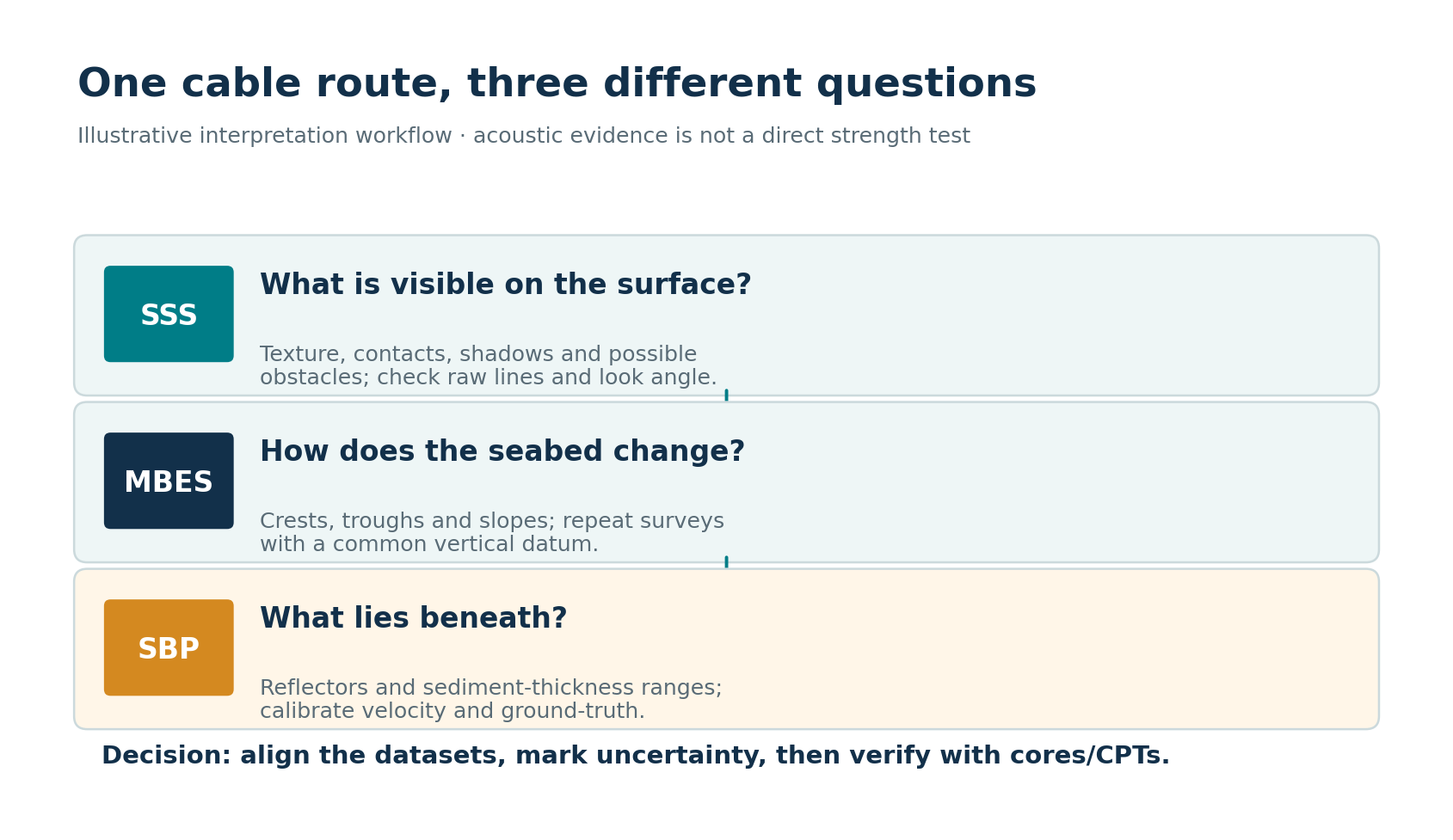
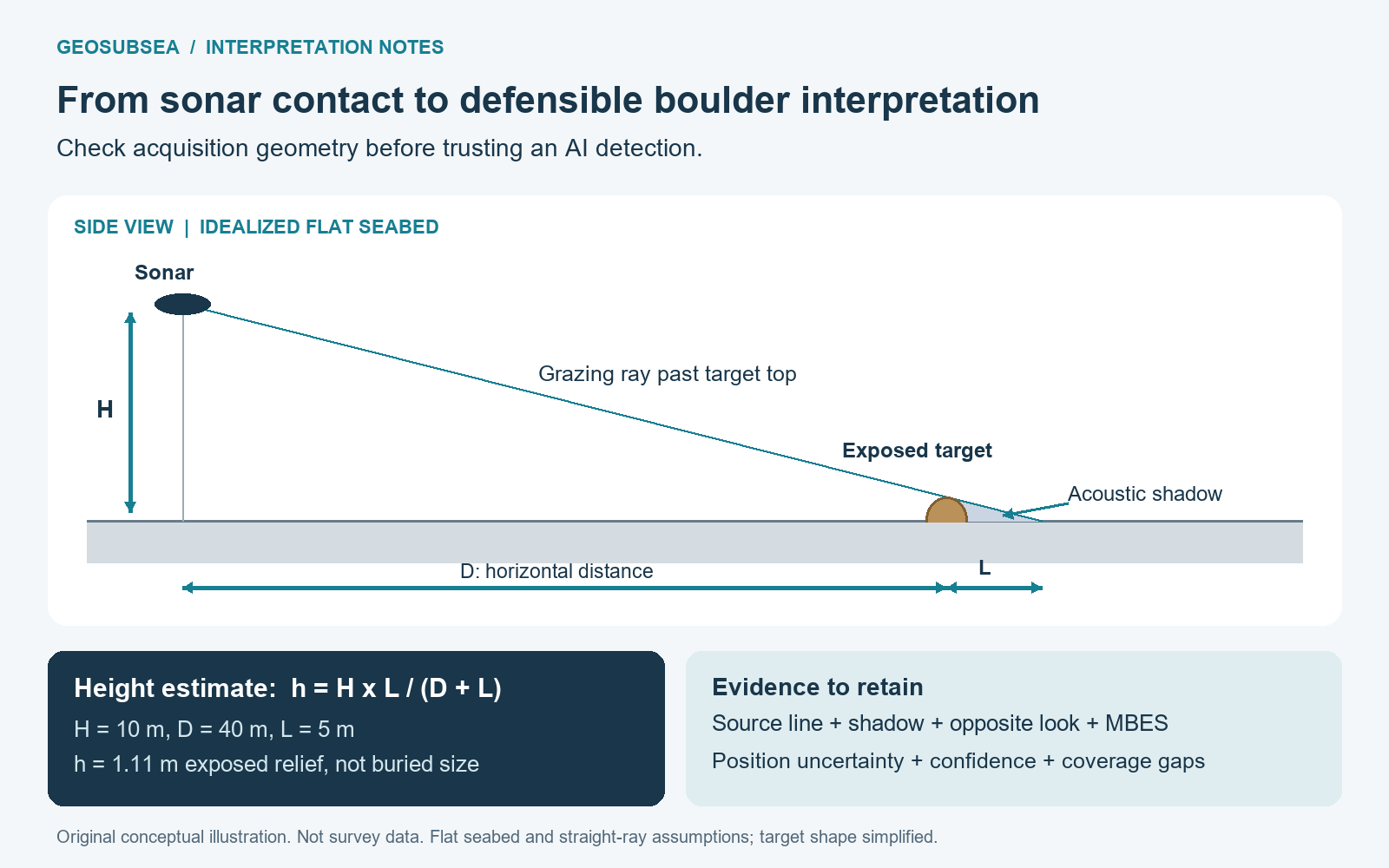
Side-scan sonar (SSS) shows acoustic texture and small surface features. A bright return next to a dark band may indicate a steep sand-wave face and its acoustic shadow; it does not measure the thickness of sand beneath that face. Return strength also changes with grazing angle, seabed roughness and processing. The Handbook of Sidescan Sonar (Blondel, 2009) and Johnson and Helferty’s geological interpretation paper both emphasise these acquisition and interpretation limits. A colour-coded mosaic alone cannot establish sediment type, mobility or trenchability.

Multibeam echo sounder (MBES) bathymetry supplies the missing shape: crest position, trough elevation, wavelength, slope and route-relative orientation. But a single bathymetric survey is a snapshot, not a migration rate. Sub-bottom profiler (SBP) sections can image the base of a surficial unit or a shallow reflector, subject to penetration and resolution. None of these acoustic measurements independently proves sediment strength; cores and cone penetration tests (CPTs) are needed to ground-truth the engineering interpretation.

A workflow that answers the burial question

First, process and quality-control each dataset before overlaying it. For SSS, review towfish position and layback, altitude, speed, slant-range correction, gain, nadir and overlapping swaths. Inspect individual lines in addition to the mosaic: seam balancing can disguise real changes, while different look directions can reverse the apparent brightness of a slope. Record coverage gaps and the smallest feature that can realistically be resolved.

Second, build a consistently referenced MBES digital terrain model. Check sound-speed corrections, tides and vertical datum, then extract crest and trough profiles along and across the proposed route. Compare repeat surveys only after matching datum, grid resolution and positional uncertainty. An apparent 0.2 m bed-level change is not evidence of migration if the combined vertical uncertainty is of the same order. Where repeat data exist, map erosion and deposition rather than assigning one rate to the whole corridor.

Third, interpret SBP on lines that cross both crests and troughs. Pick the seabed and the shallowest credible basal reflector, document where the reflector disappears, and tie picks at line intersections. Depth conversion from two-way travel time requires a defensible sediment sound speed: thickness equals velocity multiplied by two-way time divided by two. If velocity is uncertain, publish a thickness interval rather than a deceptively precise map. Acoustic blanking, multiples or poor penetration should be marked as unknown, never silently treated as a deep, soft layer.

Finally, integrate the three interpretations with samples and CPTs. Target ground truth at contrasting facies, shallow-reflector areas and proposed trenching pinch points. An SSS texture boundary may help place a sample, but a sample at one point cannot validate every similar-looking pixel across a changing acoustic geometry. Show the confidence and provenance of each mapped unit.

A transparent route-screening example

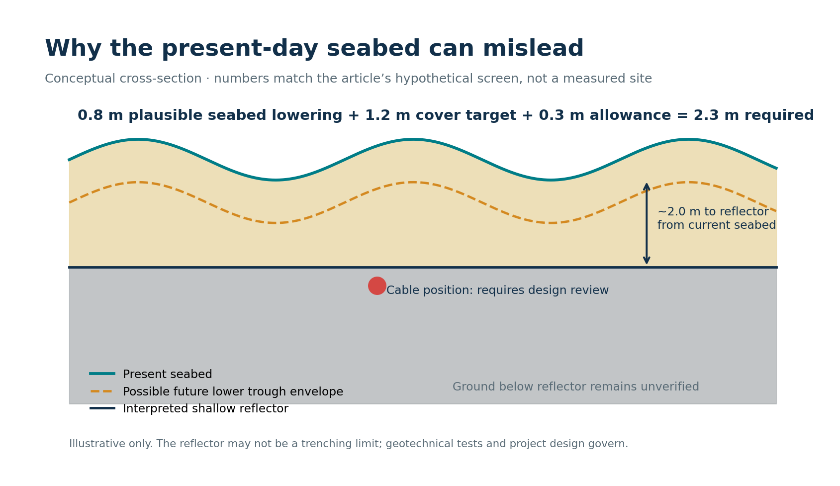
Consider a hypothetical 200 m corridor crossing a sand-wave field. A repeat MBES comparison suggests that the plausible future trough could lie 0.8 m below today’s local seabed at the critical crossing. An SBP reflector interpreted as a harder unit lies about 2.0 m below today’s seabed, with a 0.3 m depth-conversion uncertainty. Assume an engineering target of 1.2 m cover above the cable and a further 0.3 m allowance for installation and assessment uncertainty. These figures are illustrative inputs, not recommended universal design values.

A simple screen requires at least 0.8 + 1.2 + 0.3 = 2.3 m of workable depth below the current seabed. Even the nominal 2.0 m reflector is shallower than that requirement. Its uncertainty makes the decision less secure, not more favourable. A designer should test a nearby micro-route with greater interpreted sediment thickness, investigate the crossing with CPTs or cores, or assess a project-specific protection or pre-sweeping option. The final burial target and protection method belong in a cable burial risk assessment with installation engineering and environmental constraints.

This calculation is deliberately conservative but incomplete. A reflector need not be an untrenchable boundary; it may be a lithological contrast within workable sediment. Conversely, apparently thick sand may include gravel or dense material that limits the selected tool. Sand-wave migration estimates need a monitoring interval and uncertainty envelope, while future seabed change can be non-linear. Treat this screen as a reason to investigate, not as a construction specification.

Illustrative sand-wave cross-section showing possible seabed lowering, a shallow reflector and a 2.3 metre burial screen. — Figure 2. Conceptual section for the hypothetical numbers above. The red cable symbol is a decision point, not a proposed installation depth; the reflector needs geotechnical verification.

What to put on the decision map

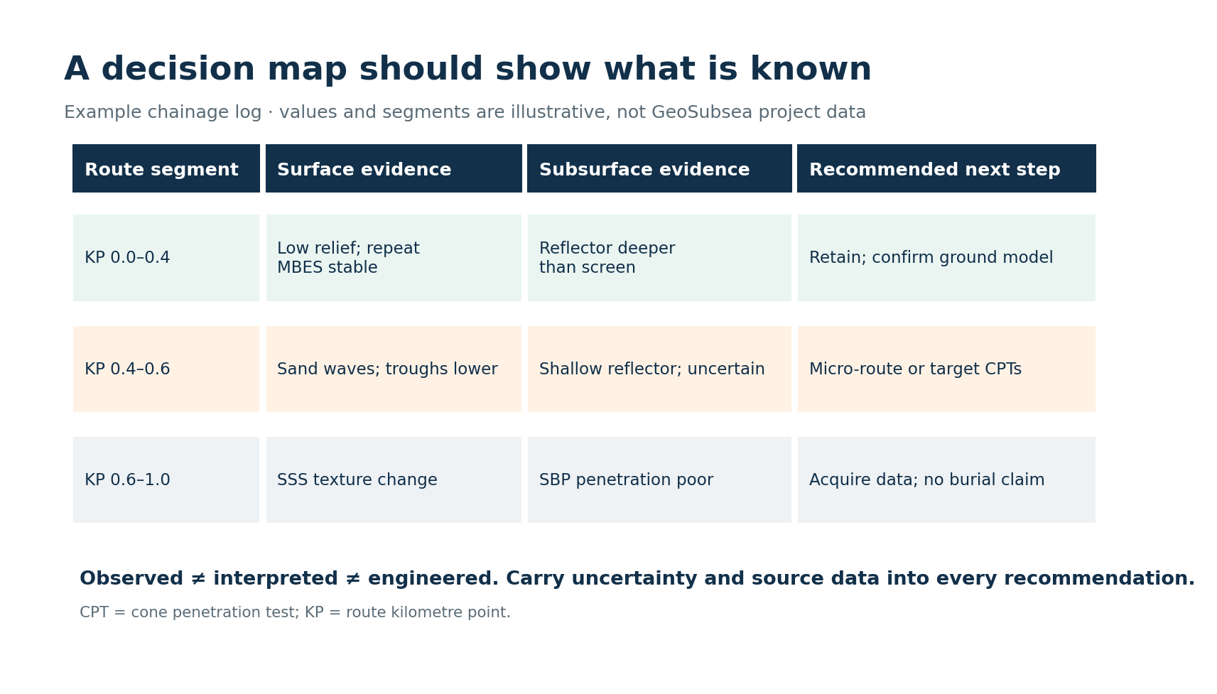
Deliver a route-aligned package with MBES crest and trough elevations, repeat-survey change and uncertainty, SSS facies and contacts, SBP reflector depth ranges, sample and CPT ties, and a chainage-based confidence log. Separate observed measurements from geological interpretation and engineering assumptions. Flag areas where poor acoustic penetration prevents a burial conclusion. For each segment, state whether to retain the alignment, move it, acquire more data, or assess mitigation. This is more useful to a cable engineer than a polished mosaic without an uncertainty trail.

Illustrative three-segment route log comparing surface data, sub-bottom evidence and next actions. — Figure 3. Example chainage log. Segment labels and recommendations are illustrative and must be replaced with project data.

A 2026 open-access routing study explicitly incorporated SBP-derived sediment thickness into offshore wind cable route analysis, addressing the weakness of routes optimised from surface conditions alone. The UK Sea Link outline cable plan likewise describes MBES for bedforms, SSS for surface features, SBP for shallow stratigraphy and targeted geotechnical checks; it discusses pre-sweeping where large sand waves cannot be avoided. The lesson is practical: survey modalities answer different questions, and the route decision depends on their agreement and on what remains uncertain.